This post presents more calculation examples for lognormal distribution, complementing and supplementing previous posts on lognormal distribution. A practice problem set is found here.
A basic introduction of the lognormal distribution is found here, with an accompanying set of practice problems found here.
Additional discussion of lognormal model is found here, using it as a model of security prices.
Lognormal Percentiles
If the mean 


Example 1
Suppose that the random variable 
The normal 90th, 95th and 99th percentiles are:


where 

First, we use tables values 


-
(1) …..

(2) …..
Divide the second equation by the first, we obtain:
-
(3) …..
Taking natural log of both sides of (3), we obtain:
-
(4) …..
(5) …..
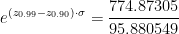
Plugging
-
(6) …..

(7) …..
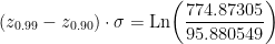
From (5) and (7), we take 

-
(8) …..
 …..(using table values)
To get a more precise answer, we use normal percentiles from the TI84+ calculator: 


-
(9) …..
 …..(using TI84+)
Order Statistics from Lognormal Samples
We use a specific lognormal distribution to demonstrate the concept. Suppose 


One important tool in learning about order statistics is through their density functions and joint density functions. When the random sample is drawn from a lognormal population, the density functions of the order statistics, though can be derived, are not easy to work with for the purpose of calculation. However, we can still evaluate probability statements about the order statistics using either a binomial calculation (when it involves only one order statistic) or a multinomial calculation (when it involves 2 or more order statistics).
The multinomial approach we use here is discussed in this previous post. The only difference is that the random samples discussed here are drawn from the lognormal distribution. A practice problem set for the multinomial approach is found here. Another set of practice problems for order statistics is found here.
We demonstrate with examples using the random sample of size 11 drawn the lognormal distribution with
Example 2
Suppose that the random variable 


Here, 


![\displaystyle \begin{aligned} P(X < 2.5)&=P[\text{Ln}(X) < \text{Ln}(2.5)] \\&=P \biggl[\frac{\text{Ln}(X)-1}{0.5} < \frac{\text{Ln}(2.5)-1}{0.5} \biggr] \\&=\Phi \biggl( \frac{\text{Ln}(2.5)-1}{0.5} \biggr) \\&=\Phi(-1.7) \\&=1-0.5675=0.4325=P \end{aligned}](https://s0.wp.com/latex.php?latex=%5Cdisplaystyle+%5Cbegin%7Baligned%7D+P%28X+%3C+2.5%29%26%3DP%5B%5Ctext%7BLn%7D%28X%29+%3C+%5Ctext%7BLn%7D%282.5%29%5D+%5C%5C%26%3DP+%5Cbiggl%5B%5Cfrac%7B%5Ctext%7BLn%7D%28X%29-1%7D%7B0.5%7D+%3C+%5Cfrac%7B%5Ctext%7BLn%7D%282.5%29-1%7D%7B0.5%7D+%5Cbiggr%5D+%5C%5C%26%3D%5CPhi+%5Cbiggl%28+%5Cfrac%7B%5Ctext%7BLn%7D%282.5%29-1%7D%7B0.5%7D+%5Cbiggr%29+%5C%5C%26%3D%5CPhi%28-1.7%29+%5C%5C%26%3D1-0.5675%3D0.4325%3DP+%5Cend%7Baligned%7D&bg=ffffff&fg=000000&s=0&c=20201002)
![\displaystyle \begin{aligned} P(X < 4)&=P[\text{Ln}(X) < \text{Ln}(4)] \\&=P \biggl[\frac{\text{Ln}(X)-1}{0.5} < \frac{\text{Ln}(4)-1}{0.5} \biggr] \\&=\Phi \biggl( \frac{\text{Ln}(4)-1}{0.5} \biggr) \\&=\Phi(0.77) \\&=0.7794=Q \end{aligned}](https://s0.wp.com/latex.php?latex=%5Cdisplaystyle+%5Cbegin%7Baligned%7D+P%28X+%3C+4%29%26%3DP%5B%5Ctext%7BLn%7D%28X%29+%3C+%5Ctext%7BLn%7D%284%29%5D+%5C%5C%26%3DP+%5Cbiggl%5B%5Cfrac%7B%5Ctext%7BLn%7D%28X%29-1%7D%7B0.5%7D+%3C+%5Cfrac%7B%5Ctext%7BLn%7D%284%29-1%7D%7B0.5%7D+%5Cbiggr%5D+%5C%5C%26%3D%5CPhi+%5Cbiggl%28+%5Cfrac%7B%5Ctext%7BLn%7D%284%29-1%7D%7B0.5%7D+%5Cbiggr%29+%5C%5C%26%3D%5CPhi%280.77%29+%5C%5C%26%3D0.7794%3DQ+%5Cend%7Baligned%7D&bg=ffffff&fg=000000&s=0&c=20201002)
The above probabilities 


Note that 


To get more precise answers, use 

 …..(using TI84+)

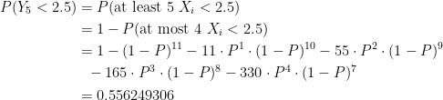
There is about a 56% chance that in a random sample of size 11 from this lognormal population, the 5th smallest sample item
Example 3
As discussed previously, the lognormal distribution has parameters
We work the first two probabilities in this example. The remaining two are done in the next example.
These probabilities involve 2 or more order statistics. One way to evaluate these probabilities is to obtain the appropriate joint density function and then integrate the joint density over an appropriate region. As mentioned earlier, the approach we take here is the multinomial approach.
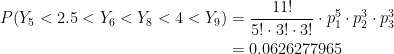
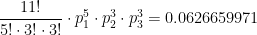
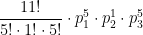
Take the first probability 


These probabilities are calculated in Example 2. The experiment is to sample from the lognormal distribution with 

When the probabilities 


 …..(using TI84+)


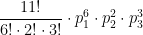
We now work the second probability 


When the probabilities
…..(using TI84+)

Example 4
We now complete Example 3 by calculating the following probabilities.
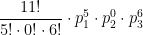
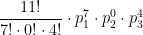
Consider the probability 


When the probabilities
…..(using TI84+)

For the probability 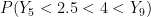


With

Example 5
Use Example 2 and Example 4 to compute the conditional probability 

 …..(using table values)

From Example 2,
Large Lognormal Samples
Independent sum of lognormal distributions is not lognormal. However if the sample is large enough, we can approximate the independent sum using the normal distribution due to the central limit theorem. We present one example.
Example 6
For a certain insurance company, insurance claims follow a lognormal distribution with parameters 

- Calculate the probability that a randomly selected claim is between 200 and 250.
- The insurance company is to process fifty claims this month. Approximate the probability that the average claim amount is 200 and 250.
For an individual claim 


For a random sample of size 50, 


We first calculate the probability 
![\displaystyle \begin{aligned} P(200<X<250)&=P[\text{Ln}(200)<\text{Ln}(X)<\text{Ln}(250)] \\&=\Phi \biggl[ \frac{\text{Ln}(250)-5}{1} \biggr]-\Phi \biggl[ \frac{\text{Ln}(200)-5}{1} \biggr] \\&=\Phi(0.52)-\Phi(0.30)\\&=0.6985-0.6179\\&=0.0806 \end{aligned}](https://s0.wp.com/latex.php?latex=%5Cdisplaystyle+%5Cbegin%7Baligned%7D+P%28200%3CX%3C250%29%26%3DP%5B%5Ctext%7BLn%7D%28200%29%3C%5Ctext%7BLn%7D%28X%29%3C%5Ctext%7BLn%7D%28250%29%5D+%5C%5C%26%3D%5CPhi+%5Cbiggl%5B+%5Cfrac%7B%5Ctext%7BLn%7D%28250%29-5%7D%7B1%7D+%5Cbiggr%5D-%5CPhi+%5Cbiggl%5B+%5Cfrac%7B%5Ctext%7BLn%7D%28200%29-5%7D%7B1%7D+%5Cbiggr%5D+%5C%5C%26%3D%5CPhi%280.52%29-%5CPhi%280.30%29%5C%5C%26%3D0.6985-0.6179%5C%5C%26%3D0.0806+%5Cend%7Baligned%7D&bg=ffffff&fg=000000&s=0&c=20201002)
The above probability using TI84+ is 0.0817076952. The following calculates the probability concerning the sample mean.
![\displaystyle \begin{aligned} P(200<\overline{X}<250)&\approx \Phi \biggl[ \frac{250-\mu_{\overline{X}}}{\sigma_{\overline{X}}} \biggr]-\Phi \biggl[ \frac{200-\mu_{\overline{X}}}{\sigma_{\overline{X}}} \biggr] \\&= \Phi \biggl[ \frac{250-e^{5.5}}{\frac{1}{\sqrt{50}} \sqrt{e^{11} (e-1)}} \biggr]-\Phi \biggl[ \frac{200-e^{5.5}}{\frac{1}{\sqrt{50}} \sqrt{e^{11} (e-1)}} \biggr] \\&=\Phi(0.12)-\Phi(-0.99)\\&=0.5478-(1-0.8389)\\&=0.3867 \end{aligned}](https://s0.wp.com/latex.php?latex=%5Cdisplaystyle+%5Cbegin%7Baligned%7D+P%28200%3C%5Coverline%7BX%7D%3C250%29%26%5Capprox+%5CPhi+%5Cbiggl%5B+%5Cfrac%7B250-%5Cmu_%7B%5Coverline%7BX%7D%7D%7D%7B%5Csigma_%7B%5Coverline%7BX%7D%7D%7D+%5Cbiggr%5D-%5CPhi+%5Cbiggl%5B+%5Cfrac%7B200-%5Cmu_%7B%5Coverline%7BX%7D%7D%7D%7B%5Csigma_%7B%5Coverline%7BX%7D%7D%7D+%5Cbiggr%5D+++%5C%5C%26%3D+%5CPhi+%5Cbiggl%5B+%5Cfrac%7B250-e%5E%7B5.5%7D%7D%7B%5Cfrac%7B1%7D%7B%5Csqrt%7B50%7D%7D+%5Csqrt%7Be%5E%7B11%7D+%28e-1%29%7D%7D+%5Cbiggr%5D-%5CPhi+%5Cbiggl%5B+%5Cfrac%7B200-e%5E%7B5.5%7D%7D%7B%5Cfrac%7B1%7D%7B%5Csqrt%7B50%7D%7D+%5Csqrt%7Be%5E%7B11%7D+%28e-1%29%7D%7D+%5Cbiggr%5D+%5C%5C%26%3D%5CPhi%280.12%29-%5CPhi%28-0.99%29%5C%5C%26%3D0.5478-%281-0.8389%29%5C%5C%26%3D0.3867+%5Cend%7Baligned%7D&bg=ffffff&fg=000000&s=0&c=20201002)
Note the difference in calculation between the probability for individual 
With 

Practice Problems
A practice problem set is found here.
Dan Ma statistical
Daniel Ma statistical
Dan Ma practice problems
Daniel Ma practice problems
Daniel Ma mathematics
Dan Ma math
Daniel Ma probability
Dan Ma probability
Daniel Ma statistics
Dan Ma statistics
Dan Ma mathematical
Daniel Ma mathematical

Tagged: Central Limit Theorem, Lognormal Distribution, Order statistics

[…] This set of practice problems is to complement a discussion on lognormal distribution (found here). […]
[…] The preceding post discusses several examples of calculation involving the lognormal distribution. This post presents another one – using the lognormal distribution as a model of prices of a financial security. Practice problems are found here. […]