This set of practice problems is to complement a discussion on lognormal distribution (found here).
Problems 8-G, 8-H and 8-I are on using the lognormal distribution as a model of security prices (see here).
Practice Problems
Practice Problem 8-A
Suppose the random variable 
Determine the 80th percentile of
Practice Problem 8-B
Suppose the random variable 


The sample median is the 6th order statistic 

Practice Problem 8-C
Same setting as in Problem 8-B. The 9th order statistic is the sample upper quartile. Determine the probability 
Practice Problem 8-D
Same setting as in Problem 8-B. Evaluate the following probabilities.


Practice Problem 8-E
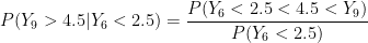
Same setting as in Problem 8-B. Evaluate the conditional probability 
Practice Problem 8-F
Insurance claims follow a lognormal distribution with parameters 

- Find the probability that a randomly selected individual insurance claim whose amount between 100 and 250.
- Find the probability that the average of the 64 claims is between 100 and 250.
Practice Problem 8-G
For a certain stock, the annual continuously compounded rate of return is modeled by a normal distribution with mean 

- Determine the probability that the stock investment will increase in value at the end of one year.
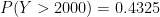
- Determine the probability that the stock investment will double in value or more at the end of one year.
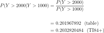
- Given that the stock investment increases in value at the end of one year, determine the probability that the investment will double in value or more.
Practice Problem 8-H
For a certain stock, the annual continuously compounded rate of return is modeled by a normal distribution with mean 

- Determine the probability that the stock investment will increase in value at the end of 5 years.
- Determine the probability that the stock investment will double in value or more at the end of 5 years.
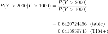
- Given that the stock investment increases in value at the end of 5 years, determine the probability that the investment will double in value or more.
Practice Problem 8-I
Use the same setting as in Problem 8-H. Determine the probability that the stock investment increases in value over each of the next 5 years.
.
.
.
.
.
.
.
.
Answers
Practice Problem 8-A
 and after rounding
80th percentile = 
80th percentile = 
Practice Problem 8-B
 (table value)

Practice Problem 8-C
 (table value)

Practice Problem 8-D
 – two cases – table value
 – two cases – TI84+


Practice Problem 8-E

Practice Problem 8-F
 (table value)
 (TI84+)


Practice Problem 8-G
 (table value)
 (TI84+)

Practice Problem 8-H
 (table value)
 (TI84+)

Practice Problem 8-H
 (table value)

Dan Ma statistical
Daniel Ma statistical
Dan Ma practice problems
Daniel Ma practice problems
Daniel Ma mathematics
Dan Ma math
Daniel Ma probability
Dan Ma probability
Daniel Ma statistics
Dan Ma statistics
Dan Ma mathematical
Daniel Ma mathematical

Tagged: Central Limit Theorem, Lognormal Distribution, Order statistics

[…] This post presents more calculation examples for lognormal distribution, complementing and supplementing previous posts on lognormal distribution. A practice problem set is found here. […]
[…] The preceding post discusses several examples of calculation involving the lognormal distribution. This post presents another one – using the lognormal distribution as a model of prices of a financial security. Practice problems are found here. […]